Through the Eye of the Eagle: Finding the Path to Soviet Supercomputing

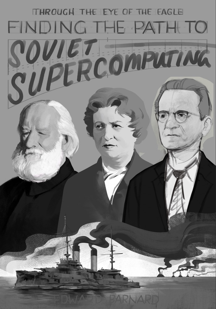
Pictured on draft cover illustration: Academician Alexei N. Krylov, Dr. Ekaterina L. Yushchenko, Academician Sergei N. Lebedev, with coal-powered battleship Orel/Eagle still afloat and in the line of battle at Tsushima, the morning of 15 May 1905 (Old Style), with battle damage.

Look Past the Surface

Like Jonathan Parshall and Anthony Tully with Shattered Sword, and David C. Evans and Mark R. Peattie with Kaigun, I looked past the standard Western computing narratives to see what others have missed. The U.S. delegation to see Soviet computing systems in May 1959, followed by the Project RAND (unrelated to Remington Rand) assessments of the 1960s, concluded that U.S. compute power was vastly superior, and stopped looking.

Thermonuclear Parity

Here is the obvious contradiction. The Soviet Union achieved thermonuclear parity during the Cold War despite having lesser compute power. The Soviet supercomputing path runs through the mathematicians. The U.S. story involves supercomputing hardware; the Soviet Union's story involves supercomputing people.

For that to be true, we need to redefine common usage of the term "supercomputing". The word came into use in the 1960s, during the Cold War. The cover story was that supercomputing involved large-scale scientific computing, because the reality remained Top Secret. We now know the primary U.S. supercomputer customers were the National Security Agency (codebreaking and signals intelligence) and the Department of Energy (the nuclear weapons laboratories).

Thus Cold War-era supercomputing supported success in those two areas. Those two areas remained State Secrets within the Soviet Union. I therefore looked at computing systems that had supercomputing capability, even in the first-generation vacuum-tube era. When I see sacrifices aimed at greater capability, I am likely seeing engineering aimed at supercomputing needs.

Supercomputing Shape

From my perspective as a Cold War participant within Cray Research, supercomputing has a recognizable shape.

One example is the "Kiev" computer (see item 3), operational in the late 1950s. It contains an internal register dedicated to holding the single return address for a function or subroutine call. At first glance that appears to be a weak design because it means no program can have recursive or reentrant code. Modern programming expects flexibility.

Non-Recursion

Here is the unstated requirement: large-memory systems enable problems to be solved that were previously intractable. Recursive programming requires memory allocated to a stack. The dedicated return address register enabled the user program to use all available memory. Primary memory was 1,024 words (about 5K bytes) that included both program and data.

The return address register is an indication of supercomputer-like design, but is not conclusive. There is more. The Kiev computer placed common subroutines in hard-wired modules. Some were permanently soldered in, and some were swappable depending on the application running. This extra complexity left all of primary memory for application use. That sacrifice in favor of enabling previously-intractable problems to be solved, is precisely what supercomputing looked like.

Hardware Loop

Another example hides within the same computing system: a pair of loop instructions (called "group instructions" by the designers).

The "Kiev" computer contains three registers dedicated to looping. The loop-initialization instruction at the start of the loop (1) sets the loop stride (e.g., increment by 5), (2) sets the current accumulated stride (e.g., 0, 5, 10, etc.), normally starting at zero, and (3) sets the exit condition (e.g., when the accumulated stride reaches 100). At that point the processor falls through to the next instruction (the loop body).

At the bottom of the loop, the loop-end instruction increments the accumulated-stride register by the stride amount (e.g., from 95 to 100), and compares the result to the exit condition register. If they are not the same, the processor jumps back to the top of the loop body (the first instruction after the initialization instruction). If they are the same, the loop-end instruction falls through to the next instruction, thus ending the loop.

Because the loop increment is handled inside the loop-exit-test instruction, the loop takes 3n+1 instructions rather than 4n instructions for a scalar product of two vectors (the "+1" instruction is that first loop initialization instruction). At first glance, that looks like a pointless distinction because it remains the same number of operations. You need to add the increment whether you do it as one instruction or two.

Here is the beauty: with first-generation computing systems, instruction fetch generally took an order of magnitude longer than register-to-register operations. This is the modern "memory latency" or "memory bandwidth" barrier to be overcome. The difference between 3n and 4n instructions executed becomes a spectacular optimization for long-running calculations.

Per-Address Indexing

However, there is another optimization hiding within the loop body. Software optimizations generally take multiple hardware instructions (with the high cost of instruction fetch), and hardware optimizations hide within the single instruction (removing the cost of instruction fetch).

Each "Kiev" computer machine instruction has the instruction purpose (opcode), and three addresses (marked I, II, III in the figure). The three addresses are generally the address of the left operand in memory, the address of the right operand in memory, and the location of where to store the result. However, each address also has a "modifiability" bit, and that bit does not mean what I expected.

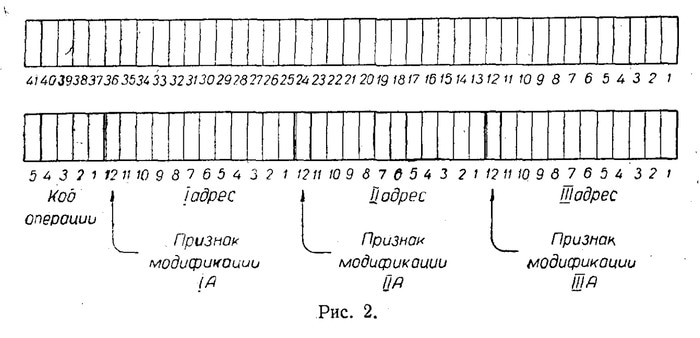
When the modifiability bit is set for any address in any instruction, the accumulated-stride value is added to the address before its use. This allows, for example, multiplying a vector by a constant: walk through the array for the left operand, fetch the constant from the same place for the right operand, and walk through the destination addresses when generating results.

This hardware-supported loop capability allows walking through arrays, lists, or more complex structures via a dictionary or registry. The hardware supports pointer arithmetic, with single, double, or higher-level address dereferencing.

Mathematical Topology Traversal

So far this sounds like traditional C programming with pointer references. It is, but that is the simple version of the capability. There is more.

Instructions and data share the same address space. The loop body can freely modify (rewrite) any instruction in memory. Specifically, the loop body can overwrite the loop initialization instruction. Then, the programmer can write the loop-end instruction to jump back to the initialization instruction rather than the loop body right after it. Remember, the initialization instruction sets up the stride, stride base, and exit condition.

How is this useful? The Kiev computer's Address Language (item 5, titled Targeted Programming, 1963) is usually described as pointer arithmetic. But, as Ekaterina L. Yushchenko (the Russian spelling of her name, common in Soviet-era sources) explains in her 1964 Doctor (Nauk) thesis (see item 6), it is implementing a topology of addresses. This ability to re-initialize the loop conditions every pass through the loop, allows the computing system to traverse a global topology with components having differing structure. Each pass sets up the conditions for the next pass.

In solving any problem, a traversal or scanning [обозревание] of the information relating to it is required. This is easily achieved in algorithms if the information is small and the connection between the elements of the set, which determines the succession operations within it, is simple. With a large volume of information and complex succession operations, in order to compose traversal schemes it is necessary to use addresses of the second and higher ranks [levels of indirection].

In [26] it is shown that by applying standard methods of encoding and schemes of surveying information via addresses of higher ranks, one can pass all the data necessary for subprograms by means of only one or two addresses that store information about the distribution of these data over addresses. (Thesis pages 21-22)

I do not have the mathematical background to explain topologies. But the people writing the thermonuclear applications, such as Dr. Mikhail Shura-Bura, did. The mathematicians did far more than overcome physical barriers in hardware. They also removed unnecessary calculations.

For example, in multiplying matrices, there is no need to multiply something by zero or one, because the result will always be zero or the starting operand. Academician Andrei Ershov's compiler removed the unnecessary calculation instructions (identity operations) entirely before run-time. With the high cost of instruction fetch, never fetching the instruction in the first place is a huge optimization.

The Battleship

All of this supercomputing requires a starting point. I picked a battleship as the starting point.

The Imperial Russian battleship Orel (Eagle in English) was one of four Borodino sister battleships that sailed from the Baltic, around Africa to the Pacific. The other three capsized, turning keel-uppermost before sinking under the waves. (English-language accounts, based on Novikoff-Priboy's novel Tsushima, are incorrect on many details important here, including manner of loss.)

Orel/Eagle's survival was due to the mathematics of naval architect Alexei N. Krylov (later known for Krylov subspace) and shipbuilder Vladimir Kostenko who served aboard Orel as a civilian crew member with rank equivalent to junior naval officer. During the long voyage, Kostenko studied Krylov's manuscript for the upcoming book on unsinkability of ships with calculated tables for flooding to compensate for battle damage (Volume XII, Part I of Krylov's Collected Works).

When Kostenko returned from captivity in 1906, the prevailing account blamed faulty ship design and engineering, rather than the naval officers, for the Tsushima disaster. Kostenko filed a detailed engineering report (expand the images to 4X or 5X to see high-resolution version) showing why Orel remained afloat despite command decisions, and that human decisions rather than engineering were the root cause of disaster. During the extremely hostile hearing, Kostenko and that paper prevailed, and Orel's officers were exonerated. That paper exists in the Yeltsin Presidential Library and serves as primary source for Orel and Krylov's mathematics.

I chose Orel as our starting point to demonstrate that Imperial Russian and Soviet mathematics dealt in consequence. Neither wind, weather, nor battle allow the rollbacks or do-overs expected with modern computing. The theory of unsinkability and Krylov's supporting mathematics determined who lived and who drowned, whether the ship floated or sank. Krylov, later Academician and General of the Fleet (флота генерал, 1916), became famous for mathematical theory, but his theory was based in hands-on practice.

On one occasion Krylov was in charge of getting newly-manufactured locomotives shipped to the Soviet Union. Loading a steamship with 85 locomotive boilers is challenging. He got down in the hold, swung the sledgehammer himself to set bracing to show the stevedore what he meant. He had already done the math. The engines loaded successfully.

The next day, Krylov's photograph appeared in the local Newcastle newspaper regarding the large order of locomotives, as "Admiral Krylov, Author of the Loading Design." (Professor Krylov's Navy, page 396, Russian-language original in Krylov's Collected Works, Volume I, Part 1)

This portrait and the caption embarrassed the stevedore to no end. He said, "I took you for a boatswain, but you are an admiral, and with your own hands, you drove the crossbar with the sledgehammer to show me what you need. You Soviets are wonderful people."

Krylov's mathematics remain relevant to this day. One example is Higham and Mary, "A New Approach to Probabilistic Rounding Error Analysis" (2019). Krylov addressed the same question in his course Lectures on Approximate Calculations (Лекции о приближенных вычислениях), Chapter V, Section 51 in 1906 (published in book form 1911).

A board of stellar Academicians gathered in 1948 to issue the multi-volume Collected Works of Krylov. I caught two numeric errors in the 1911 Lectures on Approximate Calculations, Chapter V, Section 51 (page 189), so I checked the Collected Works. The Collected Works has both errors corrected to the values I expected (page 191).

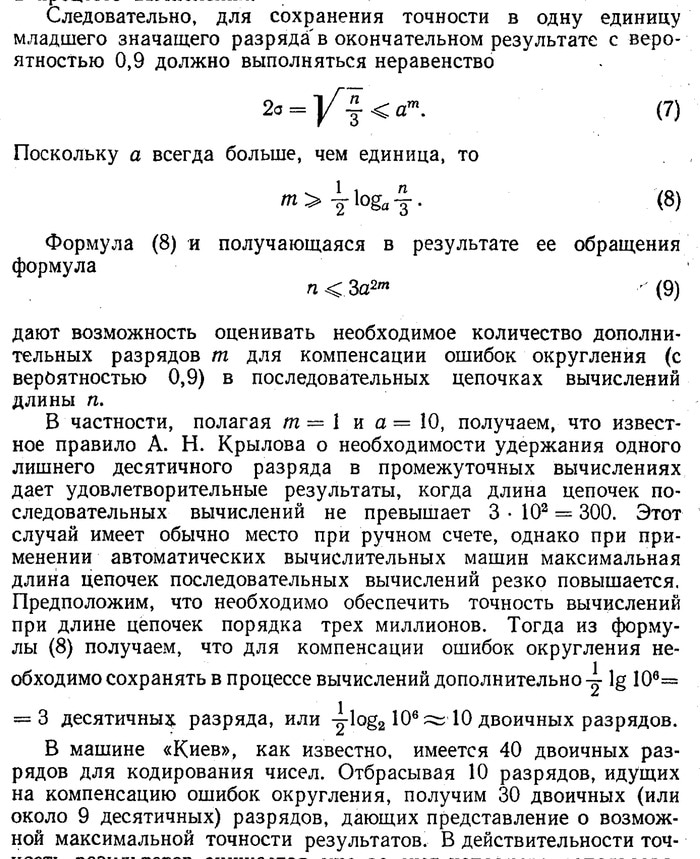
Academician Viktor Glushkov, in 1962, took Krylov's formula (crediting Krylov) for estimating accumulating rounding errors. The "Kiev" computer had 40 significant bits (plus sign bit, for 41-bit data words). He knew that Krylov taught naval engineers to use one extra decimal digit to encompass rounding errors with manual calculations. Krylov's formula showed that was valid for up to 300 consecutive calculations. (The image is from The "Kiev" Computer, page 26.)

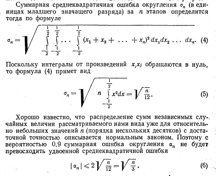
But Glushkov applied the formula to digital computing. Assuming three million intermediate calculations, how many bits should be considered corrupt (due to accumulated rounding errors) at a .9 probability? He shifted the formula to log(base 2 or base 10) notation, so that the formula would produce the estimated number of bits or decimal digits to assume corrupt. He concluded 10 bits or 3 decimal digits, leaving 30 bits of reliable precision across three million calculations. With his very next sentence he noted the danger of catastrophic loss of precision, for example from subtracting two numbers close to each other, or mismatched magnitudes. He recommended careful ordering of operations to ensure no catastrophic loss. (The image is from The "Kiev" Computer, page 27.)

This course's provocative example is that the West surfaced Krylov's rule twice in 2019: once via Higham and Mary's paper on probabilistic error analysis, and again with Sakr et al. writing about bit precision during deep-learning accumulation. Krylov's teaching on approximate calculations regained relevance because AI/ML floating-point arithmetic is not infinite precision, and therefore each calculation is an approximation.

When placing Krylov (1906), Glushkov (1962), Higham and Mary (2019), and Sakr et al. (2019) side by side, the difference is striking. All ask the same fundamental question concerning precision and validity of calculated results, state the same basic premise (rounding errors independent of each other, centered on zero, therefore tending to cancel each other out), with differing calculation models (manual calculations originating with shipbuilding; fixed-point digital arithmetic; floating-point mantissa; constrained coefficient/mantissa combinations), and differing conclusions. What, then, is the striking difference?

• Krylov and Glushkov remain anchored in physical reality and produce engineering results directly applicable to the task at hand.
• Higham and Mary begin with hardware-based premises and continue (section 3) "We now apply Theorem 2.4 within the error analysis of a variety of algorithms in numerical linear algebra." The opening sentence (section 1) addresses "the rise of large-scale, mixed-precision computations" but the ensuing discussion shifts from hardware to software, abstracting away from the hardware constraint in sharp contrast to Glushkov.
• Sakr et al. begin (abstract, first sentence) "Efforts to reduce the numerical precision of computations" based in hardware, measure and graph three specific benchmarks, state "these are very encouraging signs" (last statement before conclusion), conclude (section 6) "our theoretical concepts are application agnostic" and claim (last statement of abstract) "Overall this analysis enables precise tailoring of computation hardware to the application, yielding area- and power-optimal systems."

Both 2019 papers are well-respected, and rightly so. The striking difference is the shift away from remaining grounded in physical reality. This shift began in 1995 when we began hiding physical reality behind abstractions. We disconnected problem from solution, and both papers exemplify this shift. An entire generation has grown up on the assumption of infinite hardware availability. Not of infinite-precision hardware, but of the availability of more hardware to spin up as needed.

Unlike Soviet (and U.S.) supercomputing of the 1960s, modern AI/ML high-performance computing has become a frantic and supremely unnecessary buildout of countless new data centers: a multi-billion-dollar mistake in progress.

This century-wide comparison is not a priority dispute. Each mathematician was answering a slightly different question, demonstrating that the same invariant keeps surfacing. Technology changes, but the mathematics, and the physics, do not.

In other words, finding the path to Soviet supercomputing proves to be a fable for our times. That is how this course earns its place as part of "The HPC Tradecraft Apprenticeship". Modern AI/ML has much to learn from Soviet-era supercomputing, at a tremendous cost savings, but the modern incentive structure runs the wrong way. "Release now, patch later" is the more profitable path. Throwing in more compute power, rather than designing for efficiency, is the expected (and therefore well-funded) norm.

Organizing Theme

I organized Through the Eye of the Eagle around three specific concepts that enabled achieving thermonuclear parity during the Cold War:

• Economy of precision. Krylov's insight that a measurement only good to within 5% cannot honestly be reported to six decimal places, and his formula (derived from the Laplace theorem, direct ancestor of the Central Limit Theorem) showing how rounding error accumulates with the square root of the number of operations.
• Overcoming the barrier. The "Kiev" computer's group instructions, which fold a loop's increment-and-test into a single hardware instruction, turn 4n instructions into 3n+1 instructions for a scalar product of two vectors. That seems pointless, being the same number of operations, but in first generation computers, instruction fetch was an order of magnitude slower than register-to-register operations. The Kiev computer converted the instruction-fetch barrier into a sharp advantage.
• Economy of calculation. Academicians Gurii I. Marchuk and Andrei P. Ershov, and Dr. Mikhail R. Shura-Bura, exemplify what a computing culture builds when it invests in people rather than hardware. Ershov realized that multiplying by zero always produces zero, and multiplying by one always produces the operand, so his compiler completely removed instructions multiplying by zero or one before runtime.

Disambiguation and a Metal Bucket

I consider Through the Eye of the Eagle: Finding the Path to Soviet Supercomputing a fable for our times, with respect to modern AI/ML buildout. I should therefore note a specific limitation of frontier-class Large Language Models (specifically Claude Opus 4.8).

Typical Western narratives concerning Soviet supercomputing, and concerning details of the Battle of Tsushima in 1905, are flawed. That is why I wrote this course. I am writing from Russian-language primary sources that are apparently not present in training data. When something has no representation in training, LLMs generally do not consider possibilities regarding that fact or event, because the fact or event does not exist (from the LLM perspective).

I created the following sections as a road map providing context for what English-language online searches might turn up. Spellings will vary.

Academic Standing

The Soviet academic title "Candidate" is generally equivalent to a U.S. Ph.D. with U.S. title "Dr." The Soviet academic title "Doctor" which I generally show as "Doktor-Nauk" is a higher degree than Candidate. Doctor (Nauk) generally requires an original contribution to the science or its practice. Both generally require a thesis/dissertation defense before a board. In E.L. Yushchenko's case, her thesis was "the report on the totality of completed and published works" in lieu of an additional dissertation. This appears to be standard practice where the person's original contributions were already in published form.

Individual Soviet Socialist Republics (SSRs) had individual Academy of Sciences, abbreviated "AN". Thus "AN UkSSR" is the Academy of Sciences of the Ukrainian SSR. Individuals could be elected to the specific Academy as a "Corresponding Member", and thus a person might be described as "Corresponding Member of the AN UkSSR".

A person can also be elected a full member of the specific Academy, usually shown as "full" or "regular" member rather than "corresponding" member. A full member carries the title Academician, which is independent of awarded degrees such as Doctor. The title always ties to a specific Academy of Sciences.

During the Soviet era, there was a higher level, the Academy of Sciences of the USSR (Академия наук СССР). Both naval architect Alexei N. Krylov and computer scientist Sergei A. Lebedev were elected full members (Academicians) of the АН СССР. This higher status implied privileged access to the Soviet central political structure through various channels.

Alexei N. Krylov

Academician Alexei N. Krylov is known to LLMs and AI/ML as "Krylov subspace." Krylov subspace will probably not appear anywhere in the course on Soviet supercomputing. Take careful note of the trap: Krylov representation is skewed toward modern contemporary usage rather than the well-known tacit knowledge within the mid-20th-century Soviet Union.

Do not confuse with the other prominent Krylov who was a mathematician, Nikolai Mitrofanovich. His work had to do with simulations and algorithmic instability. N.M. Krylov is usually associated with his student Nikolai Bogoliubov and the "Krylov-Bogoliubov" school of mathematics.

As a naval instructor, A.N. Krylov decided as early as 1892 that the current texts had the primary value of being examples of how NOT to do calculations. For example, a naval shipbuilder might make a measurement, known to have a possible error factor (due to measurement) of plus or minus 5%. Calculations followed, based on that measurement, using logarithm tables accurate to six decimal places. Results were presented to the full six decimal places, completely obscuring the critical information that the original measurement had a 5% error factor.

Lacking digital computers in the 19th Century, it was common practice to use pre-calculated tables to assist pencil-and-paper engineering or physics calculations. I used such books, and a slide rule, as recently as the 1970s.

Krylov's contribution was identifying the error factor as significant context for the calculated result. This ran against tradition and shipbuilders continued to provide misleadingly-exact calculations.

Stepan Makarov

Vice-Admiral of the Russian Imperial Navy Stepan Makarov had a useful theory on the unsinkability of ships. To understand the theory, take a large metal bucket that is water-tight (waterproof). If you place it in a deep pool of water, it is probably top-heavy due to its handle. It will probably tip over, fill with water, and sink.

Instead, take the empty bucket and place a brick in it as ballast. Now, when you place it in the pool of water, it will NOT sink. If you add more bricks to it, carefully balancing so it stays upright, it will continue to float.

When will the bucket sink? When you have filled it with so many bricks that the upper rim dips below the water's surface. Then it will fill with water and sink.

If you place a brick in the bucket toward the left, the bucket will tip toward the left. On a ship this is called a list, and the tipping angle is the degree of list. You can correct the bucket's list by placing a brick toward the right, to balance the one toward the left. The bucket will now be lower in the water, but it continues to float. The bucket cannot sink until some part of the upper rim dips below the water's surface. Incoming ocean waves could cause that dip.

The bucket cannot sink so long as its rim remains completely above the water surface (including wave action). Makarov explained the same is true of a battleship. With a battleship, build a series of watertight compartments. If water comes in to a compartment on the left (due to battle damage), flood the corresponding compartment on the right to keep it upright. If the battleship sinks, the ideal is to sink fully upright. That means the ship survived as long as possible.

The other consideration is freeboard. That is the part of the metal bucket that you can see above the water. If battle damage puts holes in the freeboard, water can come in through those holes if the ship tips far enough over before it is righted by counter-flooding.

Makarov presented this theory time and time again, across decades of naval service, and was ignored.

First in late 1902, and formally in 1903, Alexei N. Krylov formally presented Makarov's theory with tables calculated for counter-flooding guidance based on the many possible combinations of battle damage. That too was ignored.

However, when a board of stellar Academicians gathered in 1948 to issue the Collected Works of Academician and General of the Fleet Alexei N. Krylov, that 1903 report with calculated tables was issued as part of Volume IX. Krylov's memoir is Volume 1, Part 1, issued 1949.